Nine Years After Darfield: When an Earthquake Drives a New Model – Part One
Delphine FitzenzDecember 05, 2019
The Source Model
The 2010 M7.1 Darfield earthquake in New Zealand started a sequence of events that propagated eastward in the Canterbury region over several years, collectively causing upward of 15 individual loss-causing events for the insurance industry. The Insurance Council of New Zealand state that the total insured loss was more than NZ$31 billion (US$19.4 billion).
With such a significant sequence of events, a lot had to be learned and reflected into earthquake risk modeling, both to be scientifically robust and to answer the new regulatory needs. GNS Science – the New Zealand Crown Research Institute, had issued its National Seismic Hazard Model (NSHM) in 2010, before the Canterbury Earthquake Sequence (CES) and before Tōhoku. The model release was a major project, and at the time, in response to the CES, GNS only had the bandwidth for a mini-update to the 2010 models, to allow M9 events on the Hikurangi Subduction Interface, New Zealand’s largest plate boundary fault, and to get a working group started on Canterbury earthquake rates.
But given the high penetration rate of earthquake insurance in New Zealand and the magnitude of the damage in the Canterbury region, the (re)insurance and regulatory position was in transition. Rather than wait for a new National Seismic Hazard Map (NSHMP) update (which is still in not available), RMS joined the national effort and started a collaboration with GNS Science as well as our own research, to build a model that would help during this difficult time, when many rebuild decisions had to be made. The RMS® New Zealand Earthquake High Definition (HD) model was released in mid-2016.
The Task Ahead
Where did we start? First, RMS experts updated the Hikurangi Subduction Interface geometry using information derived from GPS measurements (such as coupling and slow-slip event location). Examining commentary from experts in New Zealand compiled in 2005 about the 1855 Wairarapa event (near Wellington), RMS showed the likely interplay between the subduction interface and upper crust faults, in its historical event validation effort – well before this inference was made about Kaikoura (M7.8 in 2016). Providing such an event scenario for clients to run allows them to stress test their model for a type of event that now seems very likely around the Cook Strait.
RMS experts also developed and published a probabilistic method that combines geomorphology data and trench data to infer the time-dependent recurrence model for a given fault or a group of faults. The method and results for Wellington, Wairarapa and Ohariu were shared and discussed with GNS, along with their method and output for the same faults. It turns out that the local crustal faults are not dominant, as previously thought, but present the same level of risk as a M8+ on the Wellington segment of the Hikurangi subduction zone. The implied clustering of large events around the Cook Strait was also assessed and shown to compare favorably with the earthquake catalog and regional numerical models.
In the South Island, the plate boundary Alpine Fault is vital for the free movement of people, goods and electricity between the east and the west shores of the South Island. For this extensively studied fault, the RMS time-dependent model incorporated computations made using the 23 consecutive events found in trenches as well as expert knowledge on the trench environment as soon as they were published.
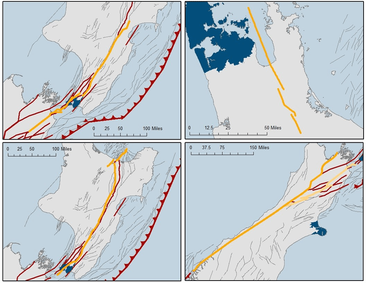
Figure One: Examples in yellow of the multi-segment or multi-fault events that were built and given rates, and are in the stochastic event set of the RMS New Zealand Earthquake High Definition (HD) model. The top and bottom left panels show events directly impacting Wellington, the top right panel shows events impacting the Auckland area, and the bottom right panel shows events that go up to but do not cross the Cook Strait (i.e., remain offshore from, but still impact Wellington).
When the updated NSHM for New Zealand was published in 2012, it did not feature any low frequency/high impact events around Wellington or Auckland. Such events are necessary to populate the tail of the exceedance probability curve to capture realistic financial reserve requirements. Since ruptures can “jump” from fault segment to nearby fault segment during the same earthquake, RMS complemented the stochastic event set with additional multi-fault ruptures. These were selected from more than 400,000 events that RMS had developed applying the Uniform California Earthquake Rupture Forecast (UCERF3) method to the 2010-2012 fault database, updated using data published at the end of the development. Only very large events were necessary since background events go up to M7.4.
RMS research was shared with GNS to help with their own research plan. Note that this effort happened as UCERF3 was still ongoing in the U.S. and before the multi-segment Kaikoura rupture happened in New Zealand. GNS experts helped select the most relevant events and assign rates, so that these events can populate the EP curve. RMS shared the challenges of using the UCERF3 methods in New Zealand with the researchers at the annual meeting of the Seismological Society of America in 2015.
But the biggest question at the time was: which rates should be used in Canterbury, where few faults are known and where the city of Christchurch needs to be rebuilt? In 2014, GNS Science scientists published a comprehensive statistical seismology study on short, medium and long-term rates for the region. Forecast rates for 2016 were still very high, due to the still large production of aftershocks. (Re)insurers are used to making business decisions based on mainshock-based models, and RMS felt it had to support the industry and use the re-assessed long-term rates. To further help clients, RMS innovated in terms of the characterization of background events (their orientation and length and spatial distribution). With nine years passed since the beginning of the sequence, there is now a much smaller difference between the current short-term rates and the new long-term rates. It was not the case back in 2015.
The RMS New Zealand Earthquake HD Model uses a simulation methodology over six year periods, that ensures that all events are sampled appropriately (annual rates from 10-9 to 10-2), and that time-dependent rates are updated year-by-year according to what was sampled in the previous year. This allows the users to notice what time series of mainshock events look like when preferential orientations for faulting are used in the model. This is relevant since many events in the Canterbury sequence are labeled as independent events by many de-clustering methods. Users can identify other possible ‘sequences’ over one to six years, in Canterbury and elsewhere, and use them for stress-tests.
Much science and know-how was developed during this project, and much outreach was and still is being done, both with the science community (in New Zealand and worldwide) and the industry. RMS remains active in the region, participating in many ongoing research projects. RMS users around the world have also been benefiting of this huge effort since RMS experts have been taking lessons learned in the region (and applied first to New Zealand) to other peril regions.
The story of the RMS New Zealand Earthquake HD Model shows the commitment of RMS to collect, produce and deliver the new understanding needed to ensure a more secure, long-term future to our clients and the communities they serve. For New Zealand, this happened through conducting reconnaissance work, taking stock of the local conditions and challenges and remaining committed to work alongside the local scientists, engineers, (re)insurers and regulators even as the country began recovery efforts during the Canterbury sequence.
One of the most striking features of the Canterbury sequence was the impact of liquefaction on losses. Click here for part two of this blog, which is centered around RMS innovation in this field.
References:
Diederichs et al., Sci. Adv. 2019; 5 : eaax5703 2 October 2019
Stirling et al, BSSA 2012, 102-4, doi: 10.1785/0120110170, August 2012
How Risk Selection in California Can Be Affected by Earthquake Source Modeling Assumptions: A Spatial Loss Correlation Perspective
There used to be several ways to ensure risk diversification in a California earthquake insurance portfolio. You could select risks on the Peninsula and risks in the East Bay; or select risks in Ventura and Orange counties; or risks in Santa Barbara and Los Angeles counties. Better yet, it was considered that selecting risks in the San Francisco Bay Area and in the Los Angeles region was a perfectly good way of achieving risk diversification. This practice was largely based on an understanding of the spatial correlation of expected loss between counties in California and selecting risks for counties which decreased loss correlations in the insured portfolio.
While California and the large-scale plate motions that it is subjected to have not changed in recent years, the way earthquake sources are modeled has. The two main areas scientists are trying to explore are: first, whether there are preferential locations in a fault network where ruptures are likely to start or stop. The second area examines what the relationship is, if any, between the timing of the latest events on a fault network and the timing of the next event that will overlap with those events. A third avenue of research that is relevant for California is the behavior of aseismic faults — faults that deform without making felt earthquakes, and what happens to them when large ruptures propagate in their direction.
RMS led a study to quantify the impact of these three major modeling assumptions on spatial loss correlations. The study used sixteen county portfolios made using the RMS Industry Exposure Database (2017), and two vintages of source model: the Uniform California Earthquake Rupture Forecast 2 and 3 (UCERF2 and UCERF3). One major conclusion was that new and different risk selection strategies would be required by the spatial loss correlation study to ensure portfolio diversification with the most recent United States Geological Survey (USGS) model (UCERF3) as compared to the previous versions of the model (i.e. UCERF1 or 2).
RMS shared this study with the broader earthquake engineering community, including those researchers who work on source models. The hope is that the study findings can inform them on the societal and commercial implications of their model assumptions, but also that it can help discriminate between source models that yield similar hazard maps at given return periods.
Figure 1: The sixteen California counties — nine in Northern California (left) and six in Southern California (right), selected for the RMS studyA Word on Loss Correlation
Common events for each portfolio drive up the value of the correlation coefficient. So, perfect correlation (+1.0) means that the list of events, event rates and secondary uncertainties between two portfolios will be identical.
___________________________
Change in spatial correlation can come from 1) change in number of events that affect both portfolios (longer/shorter ruptures than before, aka segmentation assumption), but also from 2) change in the rate of events in common (especially for different time-dependent models).
Fault Segmentation
Models up to 2008 (including UCERF2) had most ruptures start and stop at fault segment boundaries (i.e., discontinuities visible in the landscape), with a few exceptions along the San Andreas fault, for example. The most recent models (2014, UCERF3) have explored the opposite assumption: ruptures can start and stop anywhere in the fault network. In this latter case, how long and which faults the rupture is going to span depends only on a few criteria.
Instead of relying on past observed ruptures and generic assumptions about ruptures being confined to fault segments, scientists have decided to include all ruptures that could not be ruled out. That is a lot of ruptures, most of them very similar to each other, with a lot of overlap. Most of them are very long, and many involve more than one fault. Some others are shorter than individual fault segments. Since loss correlation between portfolios is driven by those events that impact both sets of exposure, one can see how this change in segmentation assumption can correlate previously uncorrelated exposures, or on the contrary reduce the correlation.
Effects of removing segment boundaries as constraints for rupture size and location:
If two counties are each close to a different fault segment and now a rupture can connect those segments, correlation is going to increase. e.g., increase in correlation between Santa Barbara and Los Angeles, for example.
On the contrary, if each end of a fault segment can rupture alone, two sets of exposure at each end of the same fault segment do not have to be correlated anymore. e.g., decrease in correlation between San Francisco county and Santa Clara county.
Time-dependent Model
Pre-UCERF3, most ruptures were confined to fault segments and the time-dependent (TD) model was applied at the scale of fault segments and only for more active and better-known faults. The largest component of the time-dependent model was a renewal model, defined by a mean recurrence time and a deviation from periodic behavior (aka aperiodicity).
The aperiodicity is not well constrained because we do not often have the dates for many consecutive large events on a fault. There are two main ways around that: 1) to use data from many faults around the world, and 2) to use numerical models simulating earthquake catalogs in a complex fault network. A third way involves using all available earthquake geology data to infer probability distributions for aperiodicity given a chosen recurrence model.
Until 2008, the Working Group on California Earthquake Probabilities (WGCEP) used the first option. The global average pointed to an aperiodicity of 0.5 being the most probable, with 0.3 (slightly more periodic) and 0.7 (slightly less periodic) also possible choices.
___________________________
Effect of high aperiodicity on few single-segment ruptures on spatial loss correlation — UCERF2 case:
Minimal effect in Southern California, slight decrease between the Peninsula counties, and slight increase in the East Bay counties (reflecting rate changes between time-independent and time-dependent perspective).
___________________________
For UCERF3, the WGCEP chose the second option, using results emerging from simulations of the fault network geometry representing California. Those exhibited a trend as a function of magnitude: the larger the magnitude, the more periodic the behavior. For most magnitudes, the aperiodicity is lower in UCERF3 than in UCERF2 (ruptures are modeled as more periodic in UCERF3 than in UCERF2).
Once coupled to the unsegmented approach, one can see how the largest, multi-segment and multi-fault ruptures become the most periodic ones as well. This does not have much impact on ruptures whose fault sections do not have a known time since the last event. However, for ruptures where we have a good understanding of time since the last event, such as the Hayward Fault, this impact is pronounced.
The probability gain relative to the time-independent model is larger for the larger magnitude, multi-segment events involving the Hayward Fault than for those events confined to the Hayward Fault alone (by virtue of the smaller aperiodicity for larger events). The same thing (but with a negative sign) happens for events overlapping with the 1906 event on the northern San Andreas Fault, In other words, the effect of time-dependence is also larger for the larger events, but the effect is to decrease their rate (the time since last event is still small compared to the mean recurrence time, an effect also called stress shadow).
___________________________
New aperiodicity scheme + TD for all fault events + unsegmented approach: UCERF3 time-dependent model relative to UCERF3 time-independent.
Loss correlations increase between the North Bay and the South Bay (through the East Bay), but they decrease between Marin County and the peninsula counties.
___________________________
Participation of the Central San Andreas Fault to Large Ruptures Linking Up Northern California Faults and Southern California Faults
Some faults are mostly aseismic, meaning they are known to deform without making felt or damaging earthquake. The San Andreas Fault, south of the San Francisco Bay Area but north of Parkfield exhibits such behavior. While scientists agree that the measured aseismic deformation across this fault does not account for all plate motion, it was previously thought that only the asperities (i.e., the parts that are stuck) could produce/participate in earthquakes. Tohoku in 2011 has shown that aseismic portions of the interface can participate in seismic ruptures if the ruptures are fast and large enough when they get to the (usually) aseismic area. In UCERF3, the WGCEP has assigned 20 percent of the accumulated moment rate for seismic events going through that section of the San Andreas fault.
Large ruptures through the central “creeping” section of the San Andreas
Events from high M5 to M>8.0 are allowed to go through that section and therefore correlate San Francisco Bay Area exposure with Los Angeles region exposure
Between San Bernardino or Riverside in the south, and Marin, San Francisco, San Mateo or Santa Clara in the north, loss correlation is up to 15 percent in the time-independent perspective and up to 10 percent in the time-dependent perspective in UCERF3*, whereas it was zero percent in previous models.
* Residential industry exposure 2017.
___________________________
To highlight and quantify those largely unstudied effects of source model assumptions on spatial loss correlations in California, RMS used RiskLink 16 (UCERF2 implementation) and RiskLink 17 (UCERF3 implementation), as well as hybrid versions between the two which kept all components uniform except the source model, and presented and published our findings at the National Conference on Earthquake Engineering in Los Angeles in June 2018. The article from the conference proceedings can be made available upon request. While the main trends are presented here, more cases and more details are discussed in the proceedings.
Notations: UCERF Uniform California Earthquake Rupture Forecast, RiskLink version 16 (based on UCERF2 in terms of California on-fault source model); RiskLink version 17 (based on UCERF3 in terms of California on-fault source model).…
Delphine Fitzenz works on earthquake source modeling for risk products, with a particular emphasis on spatio-temporal patterns of large earthquakes. Since joining RMS in 2012 after 10+ years in academia, she has strived to bring the risk and the earthquake science communities closer together through her articles and by organizing special sessions at conferences.
Delphine holds an Eng. MSc and a research MSc in geophysics from University Louis Pasteur, Strasbourg, France, and a Ph.D. from ETH Zurich, Switzerland. Her research has been on two major themes: the role of fluids and fault structure on the behavior of fault systems, and constraints on earthquake recurrence probabilistic models from individual segments to system-wide behavior. She is currently on the Technical Advisory Group for the National Seismic Hazard update project in New Zealand and on the Editorial Board of the Bulletin of the Seismological Society of America (BSSA).