The El Niño Southern Oscillation (ENSO): Discovery and Dynamics
Christopher AllenJuly 06, 2017
What is the El Niño Southern Oscillation? More conveniently known as ENSO, it is the planet’s largest source of natural climate variability on interannual time scales. ENSO describes the interaction between ocean and atmosphere in the equatorial Pacific, but the results of this interaction are global, and can last for many months. There is a good level of ENSO awareness in our industry, such as that warm phases of the oscillation (El Niño) tend to suppress Atlantic hurricane activity, and that cool phases (La Niña) tend to enhance it. But how was ENSO discovered? And how does it work?
Blanford, Todd and Walker
The term “El Niño” (Christ child) was first used by fishermen in the seventeenth century to refer to the semi-periodic emergence of unusually warm seas off the coasts of Peru and Ecuador. The name was chosen because the arrival of these warmer waters typically coincided with the Christmas period. Arguably, however, the scientific understanding of this phenomenon did not originate from South America, but from India. The failure of the Indian summer monsoon rains in 1876 and 1877 which triggered the Great Famine, prompted Henry Blanford, the Imperial Meteorological Reporter to the government of India, to look for an explanation using atmospheric pressure observations. He not only discovered that pressure was anomalously high over India, it was also simultaneously high over large parts of Asia, Australia, and the south Indian Ocean.
Blanford contacted Charles Todd, the government meteorological observer for the colony of South Australia, who realized that drought in India was also usually concurrent with drought in Australia. What was being uncovered then is what we now call teleconnections – links in climate phenomena between seemingly distant parts of the Earth.
These links can be formalized statistically, and in the 1920s, mathematician Gilbert Walker was tasked with using them to predict fluctuations in the Asian monsoon. To do this, Walker developed regression equations between Indian rainfall and other remote surface observations, such as Himalayan snowfall accumulation. Walker also came up with an index describing the long-ranging fluctuations in surface pressure that had been observed by Blanford and Todd, which he termed the “Southern Oscillation”, hence the Southern Oscillation Index (SOI).
Bjerknes: Linking the Pacific Ocean and the Southern Oscillation
None of this early work however, explained El Niño, and nor did it seek to do so. But in the late 1960s, Norwegian meteorologist Jacob Bjerknes realized that the Pacific Ocean and the Southern Oscillation were irrefutably linked.
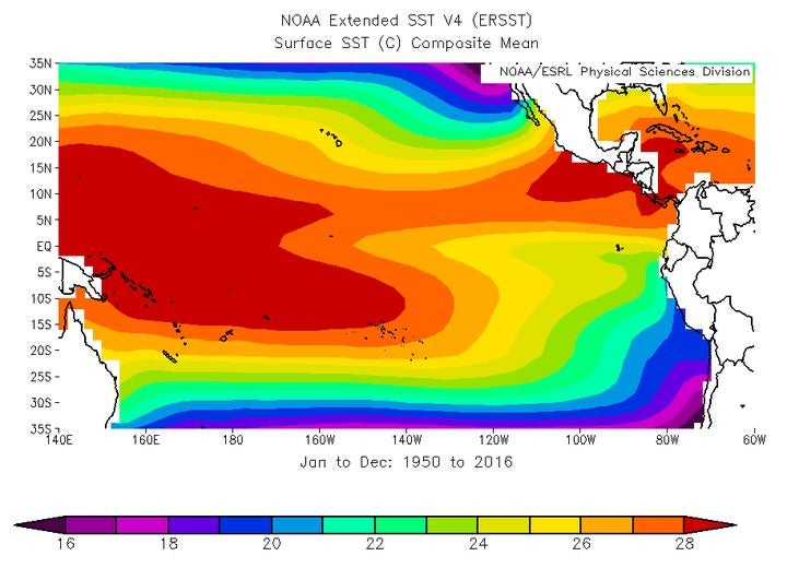
Bjerknes started with a simple but important observation, that on average, sea surface temperatures (SSTs) in the tropical east Pacific are much cooler than SSTs in the tropical west Pacific (Figure 1).
Figure 1: Average SST conditions in the tropical Pacific (1950-2016). Source: NOAA
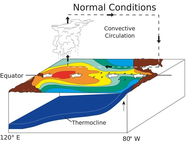
Under these conditions, known as “normal” or “neutral”, there is a thermal gradient between the two halves of the ocean basin, and as a result, winds blow from the cooler east Pacific across to the warmer west Pacific. Here, the air is heated, picks up moisture and rises, forming deep thunderstorms as the water vapor condenses. Once the air reaches the top of the troposphere, it spreads outwards back towards the east Pacific, where it cools and sinks back down over the colder water (Figure 2). Bjerknes called this atmospheric circulation loop the Walker Circulation, in honor of Gilbert Walker. Changes in the strength and position of the Walker Circulation explained fluctuations in Walker’s Southern Oscillation, and thus Bjerknes linked the Pacific Ocean with the Southern Oscillation.
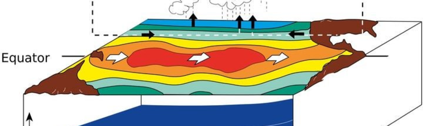
Figure 2: Normal conditions in the tropical Pacific Ocean. Source: NOAA
A further observation that Bjerknes made, was that these atmosphere and ocean conditions have a tendency to reinforce themselves. For instance, when the winds blow from east to west across the Pacific, they result in cool water being brought up from the depths towards the surface in the east Pacific (Figure 2). This increases the thermal gradient between the east and west Pacific, which strengthens the winds, which brings even more cold water up to the surface, and so the cycle intensifies. This eventually became known as the Bjerknes Feedback. When this feedback is particularly strong, and the SSTs in the eastern Pacific become significantly colder than their normally cool state, we have reached the cool phase of ENSO, known as La Niña conditions.
Explaining El Niño
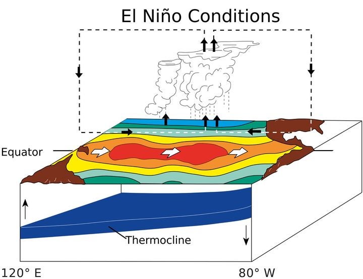
So how do we break this cycle, and end up with warm waters in the eastern Pacific, that is, El Niño conditions? Klaus Wyrtki, an oceanographer at the University of Hawaii, proposed an explanation. Tidal gauge measurements showed that when warm waters were piled up in the west Pacific, the sea level in the west Pacific was measurably higher than in the east Pacific. While winds continue to blow from east to west, this slope can be sustained, but if they relax (or reverse direction), the warm water moves downslope from the west Pacific towards the east Pacific, suppressing the upwelling of cold water and increasing SSTs, resulting in El Niño conditions (Figure 3). The anomalously warm SSTs increase deep convection and thunderstorm activity, and also shift it towards the central Pacific Ocean. This disrupts the Walker Circulation, with knock-on effects (the teleconnections) to atmospheric circulation patterns worldwide.
Figure 3: El Niño conditions in the tropical Pacific Ocean. Source: NOAA
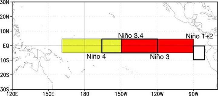
Given the complexity of the ENSO system, it is unsurprising that there are several different ways to measure it. The Southern Oscillation Index (SOI) is still used, albeit a modified version; more commonly however, SST anomalies are averaged over “boxes” that subdivide the equatorial Pacific (Figure 4). A summary of three commonly used ENSO indices is provided in Table 1.
Figure 4: ENSO “boxes”: regions over which SST anomalies are averaged. Source: NOAA
Index NameDefinitionIndex value in warm phase (El Niño)Index value in cool phase (La Niño)
Southern Oscillation Index (SOI)Standardized Tahiti sea level pressure minus Darwin sea level pressure, divided by monthly standard deviationNegativePositive
Oceanic Niño IndexSST anomaly in the Niño 3.4 box 5°N-5°S, 170°W-120°W (Figure 4)Positive (>0.5° Celsius)Negative (<−0.5° Celsius)
Multivariate ENSO IndexCombination of six variables, including sea level pressure, SST, wind speed, cloud coverPositiveNegative
Table 1: Commonly used ENSO indices
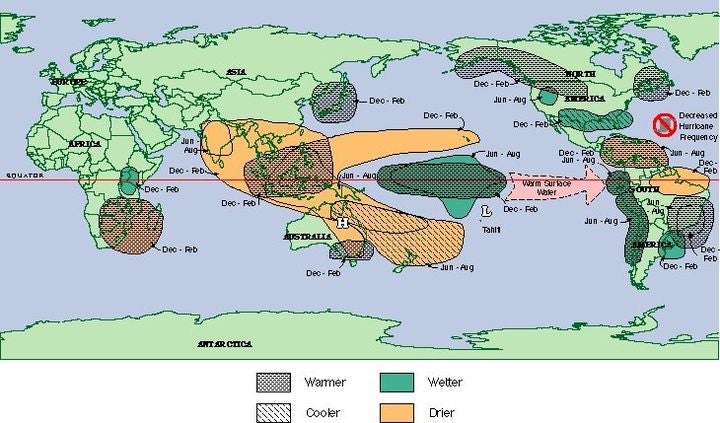
By changing pressure and wind patterns and by transmitting long-distance waves through the ocean and atmosphere, El Niño and La Niña can influence climate at great distances from the Pacific Ocean (Figure 5). For example, El Niño tends to suppress North Atlantic hurricane activity by increasing wind shear and by promoting the large-scale descent of dry air in the Main Development Region, which is discussed with relevance to this year’s hurricane season in a separate RMS blog. It also influences weather and climate more locally, such as through changing the pattern of Australian tropical cyclone activity.
Although ENSO has an irregular period of about 2-7 years, individual El Niño or La Niña events evolve in a fairly similar way, over about 12-18 months, and are somewhat coupled to the seasonal cycle. Once they have begun, it is therefore possible to forecast their evolution, which in turn makes it possible to forecast their teleconnections.
Figure 5: Typical El Niño teleconnections. Source: South Carolina State Climatology Office
Scientific understanding of ENSO began somewhat by chance with meteorological observations thousands of miles from the Pacific. Today, thanks to the existence of these very same teleconnections, our understanding of the current state and likely evolution of ENSO can be used as a tool to forecast distant climate conditions and inform decision making, several weeks or even months in advance.
Share:
You May Also Like
April 23, 2020
Severe Convective Storms in Europe: Ancient Threat, New Solution
Late May 2019 was a startlingly active period for severe convective storms (SCS) in the U.S., even after considering that May is typically one of the most active months of the year. Until about halfway through the month, the number of tornadoes being reported was around average, but after a major outbreak starting in mid-May this number shot up, bringing the year-to-date total to 1,017 tornado reports. This count is only surpassed by the extremely active years of 2008 and 2011 (Figure 1).
This year’s late May outbreak was also unusually long: by the end of Wednesday, May 29, at least eight tornadoes had been experienced each day across a record-breaking 13 consecutive days, according to preliminary data from the National Weather Service (NWS). The previous record was set in 1980, after 11 consecutive days with at least eight tornadoes.
Figure 1: Cumulative counts of tornado reports. 2019 (up to 30 May) shown in black. 2016-18 data are not plotted. Source: https://www.spc.noaa.gov/wcm/The reason this latest outbreak lasted so long was due to a particularly persistent set of atmospheric conditions favourable for SCS. A combination of a stubborn high-pressure system over the Southeast U.S. and a stationary and unusually cold trough over the Rocky Mountains, saw warm, moist air drawn from the Gulf of Mexico into the central U.S., and a strong jet stream aided the formation of supercell thunderstorms, which can generate very powerful tornadoes.
Hailstone measuring 5.5 inches found at Wellington, Texas, on May 20, 2019. Image credit: Twitter/@NWSAmarilloThe outbreak spawned tornadoes across a wide area of the U.S. (Figure 2), but most have occurred in the southern Great Plains (so-called “Tornado Alley”) and the Midwest. It has not only been tornadoes causing damage, the severe weather also generated large hail – with a 5.5 inch (14 centimeter) diameter hailstone (see above) reported in Texas, and strong straight-line winds.
Figure 2: Tornado reports by U.S. County (20-30 May 2019). Data source: NOAA (https://www.spc.noaa.gov/climo/reports/)SCS is a major contributor to annual insured losses in the United States. RMS modeling shows that average annual loss (AAL) from SCS roughly equals that from hurricanes, at around US$17 billion. Unlike losses from hurricanes, SCS losses (especially hail) accumulate over the course of a year; however, major outbreaks can make the difference between an “average” year and a significant impact to the insurance industry. Prolonged and damaging outbreaks also increase the likelihood that losses will flow through to reinsurance layers.
The most significant past tornado outbreaks, for example, the tornadoes that hit Tuscaloosa, Alabama and Joplin, Missouri in 2011, have cost single-digit billions of insured loss (USD). One particularly interesting characteristic of the late-May 2019 SCS outbreak, however, is that the damage could have been much worse. Meteorological records have been broken but – for the most part – the tornadoes avoided major cities.
That said, it will take some time before all of the claims (hail, tornado and wind) have been verified and processed, so it is too early to know what the cost of the outbreak to the insurance industry will be. It is worth noting that the SCS outbreak was accompanied by significant flooding in Arkansas, Oklahoma and Missouri, but since flood damage is not typically covered by private insurance in the U.S., if the properties were not covered by the National Flood Insurance Program (NFIP), these costs will be borne by individual home and business owners.
Below are shown some statistics and charts covering this remarkable outbreak. Unless otherwise stated, they cover the period 20-30 May 2019:
Number of Confirmed Tornadoes in the U.S. (May 16–30): ≥ 228
22 of these have not yet been given a strength rating by the National Weather Service (NWS). More tornadoes may be confirmed by the NWS as their surveys continue.
Number of EF5 Tornadoes: 0
There have been no tornadoes of the highest category on the Enhanced Fujita (EF) Scale.
Number of EF4 Tornadoes: 3
EF-4 in Dayton, Ohio
EF-4 in Linwood, Kansas
EF-4 hit Marshall, Oklahoma
…
Chris is the product manager for the RMS North America Severe Convective Storm (SCS) and Winter Storm models. He has a doctorate in Climatology from Oxford University, where he was a College Lecturer.
Apart from SCS and winter storm, he is particularly interested in hurricanes and still gets excited by his old PhD topic, Saharan dust storms. Chris is a Certified Catastrophe Risk Analyst.